Introduction to Time Series

Time series can be defined as a collection of observations from one or more variables collected in time with a certain periodicity. Study of their relationship and evolution and analyzing the behavior let us, knowing the past try to predict the future.

The fundamental characteristic is that the successive observations must have a known periodicity (hour, day, week, month, year ...) and are not independent of each other because the observations in a moment of time depend on the values ​​of the series in the past.

What are the Time Series used for?

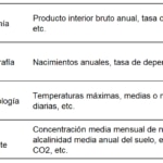
As we have said, the analysis of time series seeks to understand the past in order to make a prediction about what the future will be like. The most common fields are:

Components

To help us explain the behavior of the series over time, a descriptive study is made based on decomposing its variations into one or several basic characteristics that we call components.

The components or sources of variation that are usually considered are:

• Trend: It is the behavior or movement that occurs in the long term in relation to the average. The trend is identified with a smooth movement of the long-term series.
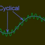
• Cyclical component: Reflects recurring behavior in higher periods, for example a year, although they do not have to be exactly periodic and often result from the superposition of different effects in different periods and often in short series they can not be separated from the trend.
• Seasonal component: Many time series have periodicity of variation in a certain period (annual, monthly ...). These types of effects are easy to understand and can be explicitly measured or even eliminated from the data set by deselecting the original series.
• Random component: are alterations of the series without a clear periodic pattern or trend. Rarely have impact on the outcome of the series and is considered to be caused by many factors small entity.

The science of data

The usual work of the data scientist has two distinct phases, the first and most important for the quality of the result is the work to be done with the data; selection of sources, cleaning and preparation of the data set or datasets and obtaining the most important features or characteristics for the second phase proceed to make the selection of the algorithms, the appropriate trainings generate the metrics and make the comparisons for finally get to generate an output of results that add value.

The first phase is inherent in the work of the data scientist and in rare cases will not occupy most of the time, being common to any Machine Learning project that is intended to be undertaken.

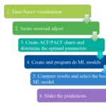
Entering already in the second phase to generate a prediction with time series, there are tasks that we must perform for each of the engines with which we will do the training and validation to finally select the best engine and make the predictions.

Auto ML

Automated learning (Auto ML) is an automated process for the optimal design of ML models that identifies the best configuration of their hyperparameters (examples: number of layers of a neural network, depth of a decision tree, etc.).

Automated learning has become a topic of considerable interest in recent years, however, contrary to what its name might imply, Auto ML is not science automated data because even for predictive tasks, Data science covers much more. Sandro Saitta (Chief Industry Advisor at the Swiss Data Science Center) commented: "The misconception comes from the confusion between the entire Data Science process and the subtasks of data preparation (feature extraction, etc.) and modeling (selection of algorithms, adjustment of hyperparameters, etc.) that I call Machine Learning ".

Still, there is no doubt that these tools are a great help and have come to the world of data science to stay.

Timecop: Time Series made simple

We have developed Timecop as an internal tool but at the same time opensource so that it can add value to many areas. The idea is to forecast timeseries without knowledge of statistics, data science or the world of machine learning. Timecop tries to introduce a series of values ​​with temporal guidelines and to obtain how they have behaved in the past, what the situation is in the present and a prediction of the future.

Timecop provides:

• A list of anomalies that have occurred in the Past: points where a high deviation occurs.
• Current state of the time series: determine if it is in an anomalous state currently
• Forecasting the timeseries: estimation of the following points in the series.

Use of Timecop

Serverless web service Restful

One of the objectives of Timecop is the easy integration with different projects where you can use your anomaly detection and prediction capabilities in a simple way and without modifications in the processes already created.

The keys accepted in the input JSON are:

• "data": series with the data of the timeseries
• "name": name of the series to work with old engines and add to existing data in timecop
• "restart"(default: False): obviate all the data stored in the series labeled by the "name" and use only the data sent in this JSON.
• _"Desvmetric"(default: 2): sensitivity for the detection of anomalies
• "future"(default: 5): number of points to be predicted.

For easy integration, Timecop is offered as a web service that offers all the possible results in a single invocation.

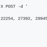
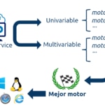
• invocation Univariable(the analysis will be made from a single time series)

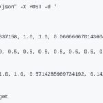
Using a POST method, a series of numbers is transmitted

• Multivariable invocation (the analysis will be based on several time series that influence the main one, on which the predictions will be made )

By means of a POST method all the series necessary for the prediction of the main series are transmitted

In both cases the response is composed of a json file containing four parts:

1.- Metrics of thewinning algorithm most accurate.

2.- List of anomalous points from the past

3.- Current status of the series (last 5 points): TRUE / FALSE and list of anomalous points

4.- Prediction of the points of the configurable series in the invocation.

Below we can see an example.

Web page

For a non-automatic use, we have developed a web page that can invoke the two URIs and visualize their response.

Once the page is open we can see the work area divided into two parts.

Data: data from the series and location of Timecop

• URL: URI invoking the Timecop service:- Univariable: http://127.0.0.1:5000/univariate- Multivariable:http://127.0.0.1:5000/multivariate
• Data set, or DataSet:

Json with the series (univariable) or set of series (multivariable) with which the web service is invoked. For greater usability we have introduced the ability to read a CSV and be able to translate it into the necessary JSON format.

If this conversion from CSV to JSON is not used, you can enter the JSONs in the following format.

* Univariable: An example of JSON can be:
{"data":[15136, 16733, 20016, 17708, 18019, 19227, 22893, 23739, 21133, 22591, 26786, 29740,15028, 17977, 20008, 21354, 19498, 22125, 25817, 28779, 20960, 22254, 27392, 29945,16933, 17892,20533, 23569, 22417, 22084, 26580, 27454, 24081, 23451, 28991, 31386, 16896, 20045, 23471, 21747, 25621, 23859, 25500, 30998, 24475, 23145, 29701, 34365, 17556, 22077, 5702,22214,26886, 23191, 27831, 35406, 23195, 25110, 30009, 36242, 18450, 21845, 26488, 22394, 28057, 25451, 24872, 33424, 24052, 28449, 33533, 37351, 19969, 21701, 26249, 24493, 24603,26485, 30723, 34569, 26689, 26157, 32064, 38870, 21337, 19419, 23166, 28286, 24570, 24001, 33151, 24878, 26804, 28967, 33311, 40226, 20504, 23060, 23562, 27562, 23940, 24584,34303, 25517, 23494, 29095, 32903, 34379, 16991, 21109, 23740, 25552, 21752, 20294, 29009, 25500, 24166, 26960, 31222, 38641, 14672, 17543, 25453, 32683, 22449, 22316]}

* Multivariable: An example with a main series (Main) and several series that help the prediction of the main series:
{"timeseries":[ {"data": [0.9500000476837158, 1.0, 1.0, 0.06666667014360428, 0.42222222685813904, 0.0833333358168602, 0.09444444626569748, 0.23333333432674408, 0.0833333358168602, 0.9833333492279053, 0.04444444552063942, 1.0, 1.0, 1.0, 1.0, 1.0, 1.0, 1.0, 1.0, 1.0, 1.0, 1.0, 1.0, 1.0, 0.08888889104127884, 1.0, 0.9277778267860413, 0.5166666507720947, 0.9666666984558105, 0.6666666865348816, 0.3333333432674408, 0.9055556058883667, 0.8277778029441833, 0.5777778029441833, 1.0, 1.0, 0.08888889104127884, 1.0, 1.0, 1.0, 1.0, 1.0, 1.0, 1.0, 1.0, 1.0, 1.0, 1.0, 0.05000000074505806, 0.5166666507720947, 1.0, 0.03888889029622078, 0.03888889029622078, 0.4166666865348816, 0.03888889029622078, 0.03888889029622078, 0.06666667014360428, 0.5777778029441833, 0.3055555522441864, 1.0]}, {"data": [0.5, 1.0, 1.0, 0.5, 0.5, 0.5, 0.5, 0.5, 0.5, 0.5, 0.5, 1.0, 1.0, 1.0, 1.0, 1.0, 1.0, 1.0, 1.0, 1.0, 1.0, 1.0, 1.0, 1.0, 0.5, 1.0, 0.5, 0.5, 0.375, 0.5, 0.5, 0.5, 0.5, 0.5, 1.0, 1.0, 0.5, 1.0, 1.0, 1.0, 1.0, 1.0, 1.0, 1.0, 1.0, 1.0, 1.0, 1.0, 0.5, 0.5, 1.0, 0.5, 0.5, 0.5, 0.5, 0.5, 0.5, 0.5, 0.5, 1.0]}], "main": [0.8571429252624512, 1.0, 1.0, 0.5714285969734192, 0.1428571492433548, 0.1428571492433548, 0.1428571492433548, 0.1428571492433548, 0.1428571492433548, 0.4285714626312256, 0.5714285969734192, 1.0, 1.0, 1.0, 1.0, 1.0, 1.0, 1.0, 1.0, 1.0, 1.0, 1.0, 1.0, 1.0, 0.8571429252624512, 1.0, 0.0, 0.1428571492433548, 0.2857142984867096, 0.1428571492433548, 0.1428571492433548, 0.1428571492433548, 0.1428571492433548, 0.1428571492433548, 1.0, 1.0, 0.8571429252624512, 1.0, 1.0, 1.0, 1.0, 1.0, 1.0, 1.0, 1.0, 1.0, 1.0, 1.0, 0.8571429252624512, 0.4285714626312256, 1.0, 0.0, 0.0, 0.1428571492433548, 0.0, 0.0, 0.0, 0.1428571492433548, 0.1428571492433548, 1.0]}

Visualization of results

The results are displayed in the same way in univariate and multivariable.

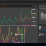
In the visualization you can see:

• the series provided (in green in the example)
• the results of the different algorithms in the test phase (dashed)
• the best existing prediction (in orange)
• anomalies (red dots)

Ready for production:

The beginning basic Timecop is generating many predictions as possible and then select the best one.

Timecop aims to compare the best models of each type of algorithm. For this, 70% of the series is taken for training and 30% for tests of all models.

Once the best model is selected with each algorithm, the chosen metric is compared (in our case, now Absolute Error Minimum, or MAE) and the prediction and anomalies of this winning model are presented.

But that search for the best algorithm involves a very high CPU time and RAM consumption that may not be required at all times.

For its use in production, it is not always necessary to search for the best algorithm, since the optimal solution is usually the reuse of the engine obtained previously. If the best algorithm is not searched, the response is made in seconds instead of minutes.

To do this, the following arguments have been included in the invocation:

• train(default: True): indicate that the best algorithm will be searched.
• restart(default: False): indicates that you do not want to add to the sent data stored values in timecop. In this way, you can restart the information that exists in timecop.

Architecture

The need to manage many timeseries in production environments in an agile way requires timecop to have a robust backend capable of being dimensioned in a simple way to support thousands of requests.

For this, Timecop has a celery backend to execute as many requests as necessary. In this way, it allows us to:

• isolate the processing in the search for the best algorithms, allowing an asynchronous response that does not penalize the performance of the platform,
• increasing the number of workers, so that the number of requests handled in a horizontal way can be increased in different machines / instances.

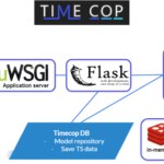
In addition to using the backend, docker image has been developed to be used very simple. The availability of a solution based on docker containers allows management adapted to the new cloud environments, horizontal scaling, versioning management, and its rapid deployment.

Algorithms used

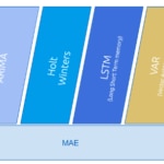
In a transparent way for the user, Timecop does the work of detecting the seasonality of the series, performing the training and validation of the different algorithms, applying the most appropriate metric, selecting the algorithm with the best results and generating the graph of exit.

Currently Timecop performs the process using the following engines; ARIMA, Holt-Winters, LSTM (Long Short Term memory) and VAR (Vector AutoRegression), these last two also applicable for multivariable series.

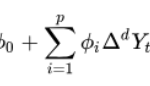
ARIMA (AutoRegressive Integrated Moving Average)

It is a dynamic model of time series that uses variations and regressions of statistical data to find patterns that allow making a prediction of the future.

It is used in seasonal time series and its use for non-series is unviable stationary.

In the ARIMA models (p, d, q), p represents the order of the autoregressive process, d the number of differences that are necessary for the process to be stationary and q represents the order of the moving average process.

The ARIMA model can be represented as follows:

Holt-Winters (Exponential Smoothing):

It’s one of the best ways of forecasting the demand of a product in a given period, Holt-Winters considers the level, trend and seasonality of a certain series of times. It incorporates a set of procedures that make up the core of the family of time series of exponential smoothing.

The same as the ARIMA model is mainly thought for series stationary, but with the advantage that its computational cost is lower.

Unlike many other techniques, the Holt-Winters model can easily adapt to changes and trends, as well as seasonal patterns. It has the advantage of being easy to adapt as new real information is available, and compared to other techniques such as ARIMA, the time needed to calculate the forecast is considerably faster

LSTM (Long Short Term memory)

The LSTM model is one of the traditional neural networks and they are widely used in prediction problems in time series because their design allows remembering information over long periods and facilitates the task of making future estimates using periods of historical records.

Unlike traditional neural networks, instead of having neurons in a classical way, LSTM networks, belonging to the Recurrent Neural Networks (RNN) class, also use their own output as input for the next prediction, in a recurrent way , thus allowing capturing the temporary component of the input. These memory blocks facilitate the task of remembering values, therefore, the stored value is not replaced (at least in the short term) iteratively over time, and the gradient term does not tend to disappear when the retrograde is applied propagation during the training process, as it happens in the use of classical neural networks.

VAR (autoregressive vector)

It’s a system of as many equations as series to be analyzed or predicted, but in which no distinction is made between endogenous and exogenous variables. Thus, each variable is explained by the delays of itself (as in an AR model) and by the delays of the other variables. A system of autoregressive equations or an autoregressive vector (VAR) is then configured. It is very useful when there is evidence of simultaneity among a group of variables, and that their relations are transmitted over a certain number of periods.

Recap

With Timecop all that is required is to introduce the numerical series to be analyzed and predicted, and to perform all the necessary previous tasks so that the data can be analyzed and processed by engines

Metrics

The key to an Auto ML system like Timecop lies in the comparison of the algorithms and trained models and the selection of the one that best suits the needs of the time series analyzed. For this, it is vital to select an accurate metric that allows a correct comparison between the different time series prediction algorithms.

Timecop performs the comparison of the different algorithms on 30% of the timeseries, selecting the engine that has the lowest MAE.

In the case of Timecop we use MAE in the training set of the time series but we provide as an output a set of the most known such as:

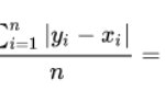
MAE (Mean Absolute Error)

The absolute average error measures the average magnitude of the errors in a set of predictions, in absolute value. It is the average on the test sample of the absolute differences between the prediction and the actual observation where all the individual differences have the same weight.

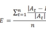
MAPE (Mean Absolute Percentage Error)

The average absolute percentage error measures the error size (absolute) in percentage terms. The fact that a magnitude of the percentage error is estimated makes it an indicator frequently used by those in charge of making forecasts due to its easy interpretation. It is even useful when the demand volume of the product is not known given that it is a relative measurement

MSE (Mean Squared Error)

The mean square error takes the distances from the predicted points to the real points (these distances are the "errors") and they are square Quadrature is necessary to eliminate any negative signs.

Having the square of the difference gives more weight to the outliers, that is, to the points with larger differences.

RMSE (Root Mean Squared Error)

RMSE is a quadratic scoring rule that also measures the average magnitude of the error. It is the square root of the average of the square differences between prediction and actual observation.

Conclusions

Timecop wants to fill a gap in the world of Auto Machine Learning to simplify the work of data scientists in time series.

It aims to reduce the non-creative work of selecting the best model according to the characteristics of the time series, leaving more time for data scientists to select the features and their integration in environments that provide the appropriate value.

It allows to perform temporary analysis in short periods of time, being able to know the anomalies and predictions of hundreds of series at the same time and opening new worlds for the comparison of evolutions of thousands and millions of series in a simple way that did not exist to date.

PD: thanks to everyone who has helped in timecop.

References

• Timecop project: https://github.com/BBVA/timecop